| 일 | 월 | 화 | 수 | 목 | 금 | 토 |
|---|---|---|---|---|---|---|
| 1 | 2 | 3 | 4 | |||
| 5 | 6 | 7 | 8 | 9 | 10 | 11 |
| 12 | 13 | 14 | 15 | 16 | 17 | 18 |
| 19 | 20 | 21 | 22 | 23 | 24 | 25 |
| 26 | 27 | 28 | 29 | 30 | 31 |
- t검정
- R4DS
- 최저 시급
- 통계오류
- 핵 개발
- 비율
- 산입 범위
- 유닛테스트
- R 프로그래밍
- 찬물샤워
- 성악설
- 통계 오류
- 비행기 추락
- 산입범위
- 조던피더슨
- 티모시페리스
- 자기관리
- 이기적 유전자
- 비선형성
- 아인슈타인
- t-test
- R 기초
- 큰수의 법칙
- 인터스텔라
- 핵개발
- 선형성
- 동전 던지기
- 최저시급 개정안
- 멘탈관리
- 수학적 사고
- Today
- Total
public bigdata
Introduction to TensorFlow in Python 정리[datacamp] 본문
Introduction to TensorFlow in Python 정리[datacamp]
public bigdata 2020. 3. 15. 19:04Part1
<Constants and variables>
train_input_fn
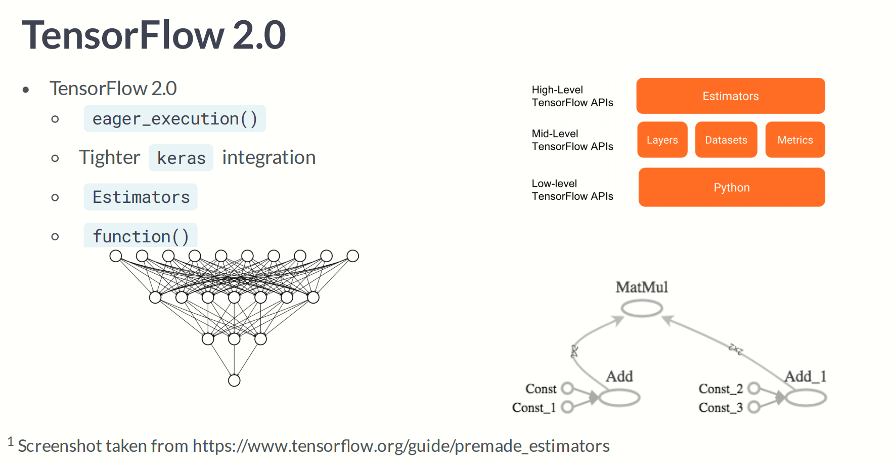
Tensorflow2.0 changes
- Eager execution by default
- Model building with Keras and Estimators
<Eager execution by default>
텐서플로의 즉시 실행은 그래프를 생성하지 않고 함수를 바로 실행하는 명령형 프로그래밍 환경입니다. 나중에 실행하기 위해 계산가능한 그래프를 생성하는 대신에 계산값을 즉시 알려주는 연산입니다
<Defining tensor in tensorflow>
import tensorflow as tf

# 0D tensor
d0 = tf.ones((1, ))

# 1D tensor
d1 = tf.ones((2,))

# 2D tensor
d2 = tf.ones((2, 2))

# 3D tensor
d3 = tf.ones((2, 2, 2))
<Defining constants in Tensorflow>
constant는 가장 간단한 종류의 tensor이다.
- Not trainable
- can have any dimension
from tensorflow import constant

# Define a 2*3 constant
a = constant(3, shape = [2, 3]) # 3으로 2행 3열 만듬 값이 부족하니까

# Define a 2*2 constant
b = constant([1, 2, 3, 4], shape = [2, 2])
<Using convenience functions to define constants>
- constant([1, 2, 3])
- zeros([2, 2])
- zeros_like(input_tensor) : 동일한 모양의 0값으로 채워진 tensor 생성
- ones([2, 2])
- ones_like(input_tensor) : 동일한 모양의 1로 채워진 tensor 생성
- fill([3, 3], 6) : 특정 값으로 채워진 tensor 생성
<Defining and initializing variables>
import tensorflow as tf

# Define a variable
a0 = tf.Variable([1, 2, 3, 4, 5, 6], dtype = tf.float32)

# Define a constant
b = tf.constant(2, tf.float32)

# compute their product
c0 = tf.multiply(a0, b) # 원소들의 곱
Tensorflow 버전 2.0에서는 데이터를 numpy 배열 또는 tensorflow 상수 객체로 사용할 수 있습니다. 상수(constant)를 사용하면 해당 객체로 수행 된 모든 작업이 tensorflow에서 수행됩니다.
<Applying the addition operator>
from tensorflow import constant, add

# Define 2-dimensional tensors
A2 = constant([[1, 2], [3, 4])
B2 = constant([[5, 6], [7, 8])

# Perfom tensor addition with add()
C2 = add(A2, B2)- add() operation performs element-wise addition with two tnesors (요소별 덧셈을 한다)
- Element-wise addition requires both tnesors to have the same shape
<How to perform multiplication in Tensorflow>
- The matmul(A, B) operation multiplies A by B (행렬 곱)
<Summing over tensor dimensions>
The redeuce_sum() operator sums over the dimensions of a tensor
- reduce_sum(A) sums over all dimensions of A
- reduce_sum(A, i) sums over dimension i
from tensorflow import ones, reduce_sum

# Define a 2*3*4 tensor of ones
A = ones([2, 3, 4])

# Sum over all dimensions
B = reduce_sum(A)

# Sum over dimensions 0, 1 and 2
B0 = reduce_sum(A, 0)
B0 = reduce_sum(A, 1)
B0 = reduce_sum(A, 2)
<Advanced operations>
In this lesson, we explore advanced operations
- gradient(), reshape(), and random()
<Overview of advanced operations>
- gradient() : compute the slope of a function at a point (한 점에서 함수의 기울기 계산)
- reshape() : Reshapes a tensor (e.g. 10*10 to 100*1)
- random() : Populate tensor with entries drawn from a probability distribution
<Gradients in Tensorflow>
import tensorflow as tf

# Define x
x = tf.Variable(-1.0)

# Define y within instance of GradientTape
with tf.GradientTape() as tape:
	tape.watch(x)
    y = tf.multiply(x, x)

# evaluate the gradient of y at x = -1
g = tape.gradient(y, x)
print(g.numpy())
> -2.0
대략적으로 무슨 말인지는 알겠지만, 자세히 이해가 되지는 않는다. 어쨋든 x = -1 지점에서의 기울기 -2.0을 구했다. 기울기가 음수면 x값을 늘리고, 양수면 x 값을 줄여서 loss를 감소 시킬수 있다.
<How to reshape a grayscale image>
import tensorflow as tf

# Generate grayscale image
gray = tf.random.uniform([2,2], maxval= 255, dtype = 'int32')

# Reshape grayscale image
gray = tf.reshape(gray, [2*2, 1])
<How to reshape a color image>
import tensorflow as tf

# Greverate color image
color = tf.random.uniform([2, 2, 3], maxval=255, dtype = 'int32')

# Reshape color image
color = tf.reshape([2*2, 3])
위 코드에서 [2, 2, 3]은 2행 2열이 3개인 상태를 의미한다 이것을 2차원으로 변경하면 [2*2, 3]이 된다.
Part2
<Input data>
Simple option used in this chapter
- Import data using pandas
- Convert data to numpy array
- Use in tensorflow without modification - 수정없이 텐서플로우에서 사용가능하다
# Import numpy and pandas

import numpy as pd

import pandas as pd


# Load data from csv

housing = pd.read_csv('kc_housing.csv')


# Convert to numpy array

housing = np.array(housing)
Pandas로는 추가적으로 read_json, read_html, read_excel등을 활용할 수 있다.
<Setting the data type>
# Load KC dataset

housing = pd.read_csv('kc_housing.csv')


# Convert price column to float32

price = np.array(housing['price'], np.float32)


# Convert waterfront column to boolean

waterfront = np.array(housing['waterfront'], np.bool
아래와 동일
# Convert to price column to float32

price = tf.cast(housing['price'], tf.float32)


# Convert warterfront column to boolean

waterfront = tf.cast(housing['waterfront'], tf.bool)
<Loss functions>
Loss functions are accessible from tf.keras.losses()
- tf.keras.losses.mse
- tf.keras.losses.mae
- tf.keras.losses.Huber - 요건 뭐지.
<Why do we care about loss functions?>
MSE
- Strongly penalizes outliers - 특이치에 강하게 페널티를 준다??????
- High sensitivity near minimum - 최소치에 가까운 높은 민감도를 가진다.
MAE
- Scale linearly with size of error - 오류 크기에 따라 선형적으로 확장????
- Low sensitivity near minimum - 최소치에서 낮은 민감도를 보인다.???
Huber
- Similar to MSE near minimum
- Similar to MAE away from minimum - MSE가 최소값에서 떨어져 있는 것과 유사하다.
<Defining a loss function>
## example1 ##
# Import Tensorflow under standard alias
import Tensorflow as tf

# Conpute the MSE loss
loss = tf.keras.losses.mse(target, predictions)
아래 코드와 동일(predictions 부분만 추가)
## example2 ##

# Define a linear regression model
def linear_regression(intercept, slope = slope, features = features):
	return intercept + features * slope

# Define a loss function to compute the MSE
def loss_function(intercept, slope, targets = targets, features = features):
	# Compute the predictions for a linear model
    predictions = linear_regression(intercept, slope)

    # Return the loss
    return tf.keras.losses.mse(targets, predictions)

# Compute the loss for test data inputs
loss_function(intercept, slope, test_targets, test_features)

# Compute the loss for default data inputs
loss_function(intercept, slope)
위에 코드에서 intercept, slope는 임의의 숫자가 지정된 상태에서 실행하는 코드이다. 현재까지는 최적화 과정이 없고 임의의 intercept, slope를 던져 생성된 모델과 targets와의 mse만 구하는 코드이기 때문에 intercept, slope를 tf.Constant, tf.Variable일 필요가 없다. 여기서는 임의의 스칼라, tf.Variable, tf.tensor든 무엇이든지 상관이 없다.
<Linear regression in Tensorflow>
# Define the targets and features
price = np.array(housing['price'], np.float32)
size = np.array(housing['sqft_living'], np.float32)

# Define the intercept and slope
intercept = tf.Varaibel(0.1, np.float32)
slope = tf.Variable(0.1, np.float32)

# Define a linear regression model
def linear_regression(intercept, slope, features = size):
	return intercept + features*slope

# Compute the predicted values and loss
def loss_function(intercept, slope, targets = price, features = size):
	predictions = linear_regression(intercept, slope)
    return tf.keras.losses.mse(targets, predictions)

# Define an optimization operation
opt = tf.keras.optimizers.Adam()

# Minimize the loss function and print the loss
for j in range(1000):
	opt.minimize(lambda: loss_function(intercept, slope), var_list = [intercept, slope]) # 이런식으로 lambda를 지정하는 이유가 뭔가
    print(loss_function(intercept, slope))

# print the trained parameters
print(intercept.numpy(), slope.numpy())
<Batch training>
- pd.read_csv() allows us to load data in batches
- chunksize parameter provides batch size
# Import pandas as pd
import pandas as pd
import numpy as np

# Load data in batches
for batch in pd.read_csv('kc_housing.csv', chunksize = 100):
	# Extract price column
    price = np.array(batch['price'], np.float32)

    # Extract size column
    size = np.array(batch['size'], np.float32)
<Training a linear model in batches>
# Import tensorflow, pandas, and numpy
import tensorflow as tf
import pandas as pd
import numpy as np

# Define trainable variables
intercept = tf.Variable(0.1, tf.float32)
slope = tf.Variable(0.1, tf.float32)

# Define the model
def linear_model(intercept, slope, features):
	return intercept + slope * features

# Compute predicted values and return loss function
def loss_function(intercept, slope, targets, features):
	predictions = linear_model(intercept, slope, features)
    return tf.keras.losses.mse(targets, predictions)

# Define optimization operation
opt = tf.keras.optimizers.Adam()

# Load the data in batches from pandas
for batch in pd.read_csv('kc_housing.csv', chunksize = 100):
	# Extract the targets and feature columns
    price_batch = np.array(batch['price'], np.float32)
    size_batch = np.array(batch['lot_size'], np.float32)

    # Minimize the loss function
    opt.minimizer(lambda: loss_fucntion(intercept, slope, price_batch, size_batch),
    									var_list = [intercept, slope])

# print parameter values
print(intercept.numpy(), slope.numpy())
opt.minimizer 부분에서 var_list 인자는 loss_function에서 최적화 할 변수를 알려주는 역할을 한다.
<Full sample versus batch training>
- Full Sample -
- One update per epoch
- Accepts dataset without modification
- Limited by memory
- Batch Training -
- Multiple updates per epoch
- Requires division of dataset
- No limit on dataset size
Part3
<A simple dense layer>
## Low level API ##

import tensorflow as tf

# Define inputs(features)
inputs = tf.constant([1, 35])

# Define weights
weight = tf.Varaible([[-0.05], [-0.01]])

# Define the bias
bias = tf.Variable([0.5])

# Multiply inputs (features) by the weights
product = tf.matmul(inputs, weights)

# Define dense layer
dense = tf.keras.activations.sigmoid(product+bias)
## High level ##
import tensorflow as tf
# Define input (features) layer
inputs = tf.constant(data, tf.float32)
# Define first dense layer
dense1 = tf.keras.layers.Dense(10, activation = 'sigmoid')(inputs)
# Define second dense layer
dense2 = tf.keras.layers.Dense(5, activation = 'sigmoid')(dense1)
# Define output (predictions) layer
outputs = tf.keras.layers.Dense(1, activation = 'sigmoid')(dense2)<Activation functions>
Linear : Matrix multiplication --> 행렬의 곱은 선형결합이다.
Nonlinear : Activation function --> 활성화 함수가 필요한건. 행렬의 곱이 선형이기 때문에 많은 수의 차원과 노드를 통한 복잡한 모델이 의미가 있으려면 복잡한 구조인 비선형 구조를 학습할 수 있어야 하기에 활성화 함수가 필요하다.
<The sigmoid activation function>
- Binary classification
- Low-level : tf.keras.activations.sigmoid()
- High-level : sigmoid
<The relu activation function>
- Hidden layers
- Low-level : tf.keras.activations.relu()
- High-level : relu
<The softmax activation function>
- Output layer(>2 classes)
- High-level : tf.keras.activations.softmax()
- Low-level : softmax
<Activation functions in neural networks>
import tensorflow as tf

# Define input layer
inputs = tf.constant(borrow_features, tf.float32)

# Define dense layer 1
dense1 = tf.keras.layers.Dense(16, activation = 'relu')(inputs)

# Define dense layer 2
dense2 = tf.keras.layers.Dense(8, activation = 'sigmoid')(dense1)

# Define dense layer 3
dense3 = tf.keras.layers.Dense(4, activation = 'softmax')(dense2)
위 코드가 이해가 안될 때는 노트에 노드를 그리고 그에 대응되는 행렬을 그려보도록 하자. input의 모양은 그대로이고, 그에 대응되는 weight는 노드 갯수만큼 열이 생성되고 하나의 열은 input행렬의 열의 갯수와 대응된다.
<The gradient descent optimizer>
Stochastic gradient descent(SGD) optimizer
- tf.keras.optimizers.SGD()
- learning_rate
- Simple and easy to interpret
<The RMS prop optimizer>
Root mean squared (RMS) propagation optimizer
- Applies different learning rates to each feature
- tf.keras.optimizers.RMSprop()
- learning_rate
- momentum
Gradient Descent Optimization Algorithms 정리
Neural network의 weight을 조절하는 과정에는 보통 ‘Gradient Descent’ 라는 방법을 사용한다. 이는 네트워크의 parameter들을 $\theta$라고 했을 때, 네트워크에서 내놓는 결과값과 실제 결과값 사이의 차이를 정의하는 함수 Loss function $J(\theta)$의 값을 최소화하기 위해 기울기(gradient) $\nabla_{\theta} J(\theta)$를 이용하는 방법이다. Gradient Descent에
shuuki4.github.io
- decay : momentum, decay 아직 둘다 무슨뜻인지 모르겠다.
- Allow for momentum to both build and decay
<The adam optimizer>
Adaptive moment (adam) optimizer
- tf.keras.optimizers.Adam()
- learning_rate
- beta1
- performs well with default parameter values : 기본 매개변수 값으로도 잘 수행된다.
<A complete example>
import tensorflow as tf

# Define the model function
def model(bias, weights, features = borrower_features):
	product = tf.matmul(features, weights)
    return tf.keras.activations.sigmoid(product+bias)

# Compute the predicted values and loss
def loss_function(bias, weights, targets = default, features = borrow_features):
	predictions = model(bias, weights)
    return tf.keras.losses.binary_crossentropy(targets, predictions)

 # Minimize the loss function with RMS propagation
 opt = tf.keras.optimizers.RMSprop(learning_rate=0.01, momentum = 0.9)
 opt.minimize(lambda : loss_function(bias, weights), var_list = [bias, weights])
이런식으로도 되네
# Initialize x_1 and x_2
x_1 = Variable(0.05,float32)
x_2 = Variable(0.05,float32)

# Define the optimization operation for opt_1 and opt_2
opt_1 = keras.optimizers.RMSprop(learning_rate=0.01, momentum=0.99)
opt_2 = keras.optimizers.RMSprop(learning_rate=0.01, momentum=0.00)

for j in range(100):
	opt_1.minimize(lambda: loss_function(x_1), var_list=[x_1])
    # Define the minimization operation for opt_2
	opt_2.minimize(lambda: loss_function(x_2), var_list = [x_2])

# Print x_1 and x_2 as numpy arrays
print(x_1.numpy(), x_2.numpy())
<Training a network in Tensorflow>
Often need to initialize thousands of variables
- tf.ones() may perform poorly : 성능이 저하될 수 있다?
- Tedious and difficult to initialize variables individually : 변수를 개별적으로 초기화하는 것이 지루하고 어렵습니다?
Alternatively, draw initial values from distribution
- Normal
- Uniform
- Glorot initializer
<Initializing variables in Tensorflow>
## 랜덤하게 가중치 초기화하는 방법1 ##
import tensorflow as tf

# Define 500*500 random normal variable
weights = tf.Variable(tf.random.normal([500, 500]))

# Define 500*500 truncated random normal variable
weights = tf.Variable(tf.random.truncated_normal([500, 500]))


## 랜덤하게 가중치 초기화하는 방법2 ##
# Define a dense layer with the default initializer
dense = tf.keras.layers.Dense(32, activation = 'relu')

# Define a dense layer with the zeros initializer
dense = tf.keras.layers.Dense(32, activation = 'relu', kernel_initializer = 'zeros')
<Implementing dropout in a network>
import numpy as np
import tensorflow as tf

# Define input data
inputs = np.array(borrower_features, np.float32)

# Define dense layer1
dense1 = tf.keras.layers.Dense(32, activation='relu')(inputs)

# Define dense layer2
dense2 = tf.keras.layers.Dense(16, activation='relu')(dense1)

# Apply dropout operation
droupout1 = tf.keras.layers.Dropout(0.25)(dense2)

# Define output layer
outputs = tf.layers.Dense(1, activation = 'sigmoid')(droupout1)
아래는 practice 코드 참고할만
# Define the layer 1 weights
w1 = Variable(random.normal([23, 7]))

# Initialize the layer 1 bias
b1 = Variable(ones([7]))

# Define the layer 2 weights
w2 = Variable(random.normal([7, 1]))

# Define the layer 2 bias
b2 = Variable(0.0)

# Define the model
def model(w1, b1, w2, b2, features = borrower_features):
	# Apply relu activation functions to layer 1
	layer1 = keras.activations.relu(matmul(features, w1) + b1)
    # Apply dropout
	dropout = keras.layers.Dropout(0.25)(layer1)
	return keras.activations.sigmoid(matmul(dropout, w2) + b2)

# Define the loss function
def loss_function(w1, b1, w2, b2, features = borrower_features, targets = default):
	predictions = model(w1, b1, w2, b2)
	# Pass targets and predictions to the cross entropy loss
	return keras.losses.binary_crossentropy(targets, predictions)

# Train the model
for j in range(100):
    # Complete the optimizer
	opt.minimize(lambda: loss_function(w1, b1, w2, b2),
                 var_list=[w1, b1, w2, b2])

# Make predictions with model
model_predictions = model(w1, b1, w2, b2, test_features)

# Construct the confusion matrix
confusion_matrix(test_targets, model_predictions)
<The sequential API>
- Input layer
- Hidden layers
- Output layer
- Ordered in sequence
<Building a sequential model>
# Import tensorflow
from tensorflow import keras

# Define a sequential model
model = keras.Sequential()

# Define first hidden layer
model.add(keras.layers.Dense(16, activation = 'relu', input_shape=(28*28, ))) # input 노드 784개라 생각하면 될듯

# Define second hidden layer
model.add(keras.layers.Dense(8, activation = 'relu'))

# Define output layer
model.add(keras.layers.Dense(4, activation = 'softmax'))

# Compile the model
model.complie('adam', loss = 'categorical_crossentropy')

# Summarize the model
print(model.summary())
<Using the functional API>
# Import tensorflow
import tensorflow as tf

# Define model 1 input layer shape
model1_inputs = tf.keras.Input(shape = (28*28, ))

# Define model 2 input layer shape
model2_inputs = tf.keras.Input(shape = (10, ))

# Define layer 1 for model 1
model1_layer1 = tf.keras.layers.Dense(12, activation = 'relu')(model1_inputs)
# Define layer 2 for model 1
model1_layer2 = tf.keras.layers.Dense(4, activation = 'softmax')(model1_layer1)

# Define layer 1 for model 2
model2_layer1 = tf.keras.layers.Dense(8, activation = 'relu')(model2_inputs)
# Defien layer 2 for model 2
model2_layer2 = tf.keras.layers.Dense(4, activation = 'softmax')(model2_layer1)

# Merge model 1 and model 2
merged = tf.keras.layers.add([model1_layer2, model2_layer2])

# Define a functional model
model = tf.keras.Model(inputs = [model1_inputs, model2_inputs], outputs=merged)

# Compile the model
model.compile('adam', loss = 'categorical_crossentropy')
<아래 코드를 보니 drop_out이 어떻게 적용되는지 알 수 있을것 같다>
# Define the first dense layer
model.add(keras.layers.Dense(16, activation='sigmoid', input_shape = (784, )))

# Apply dropout to the first layer's output
model.add(keras.layers.Dropout(0.25))

# Define the output layer
model.add(keras.layers.Dense(4, activation = 'softmax'))

# Compile the model
model.compile('adam', loss='categorical_crossentropy')

# Print a model summary
print(model.summary())
Part4
<Training and validation with keras>
- Load and clean data
- Define model
- Train and validate model
- Evaluate model
<How to train a model>
# Import tensorflow
import tensorflow as tf

# Define a sequential model
model = tf.keras.Sequential()

# Define the hidden layer
model.add(tf.keras.layers.Dense(16, activation = 'relu', input_shape = (784,)))

# Define the output layer
model.add(tf.keras.layers.Dense(4, activation = 'softmax'))

# Compile model
model.compile('adam', loss = 'categorical_crossentropy')

# Train model
model.fit(image_featuers, image_labels)
<The fit() operation>
required arguments
- features
- labels
Many optional arguments
- batch_size
- epochs
- validation_split
# Define sequential model
model = keras.Sequential()

# Define the first layer
model.add(keras.layers.Dense(1024, activation = 'relu', input_shape = (784, )))

# Add activation function to classifier
model.add(keras.layers.Dense(4, activation='softmax'))

# Finish the model compilation
model.compile(optimizer=keras.optimizers.Adam(lr=0.01),
              loss='categorical_crossentropy', metrics=['accuracy'])

# Complete the model fit operation
model.fit(sign_language_features, sign_language_labels, epochs=200, validation_split=0.5)
## 위 코드와 무관 ##
# Evaluate the small model using the train data
small_train = small_model.evaluate(train_features, train_labels)
# Evaluate the small model using the test data
small_test = small_model.evaluate(test_features, test_labels)
# Evaluate the large model using the train data
large_train = large_model.evaluate(train_features, train_labels)
# Evaluate the large model using the test data
large_test = large_model.evaluate(test_features, test_labels)
# Print losses
print('\n Small - Train: {}, Test: {}'.format(small_train, small_test))
print('Large - Train: {}, Test: {}'.format(large_train, large_test))<Model specification and training>
- Define feature columns
- Load and transform data
- Define an estimator
- Apply train operation
# Import tensorflow under its standard alias
import tensorflow as tf

# Define a numeric feature column
size = tf.feature_column.numeric_column("size")

# Define a categorical feature column
rooms = tf.feature_column_categorical_column_with_vocabulary_list("rooms", ["1", "2", "3", "4", "5"])

# Create feature column list
features_list = [size, rooms]
# Define a matrix feature column
feature_list = [tf.feature_column.numeric_column('image', shape =(784,))]위 두가지 코드는 실제로 데이터를 생성한 것은 아니고 객체만 생성해서 list에 저장한 것으로 보인다.
위 코드를 종합하면 아래 코드와 같다.
# Define feature columns for bedrooms and bathrooms
bedrooms = feature_column.numeric_column("bedrooms")
bathrooms = feature_column.numeric_column('bathrooms')

# Define the list of feature columns
feature_list = [bedrooms, bathrooms]

def input_fn():
	# Define the labels
	labels = np.array(housing['price'])
	# Define the features
	features = {'bedrooms':np.array(housing['bedrooms']),
                'bathrooms':np.array(housing['bathrooms'])}
	return features, labels

# Define the model and set the number of steps
model = estimator.DNNRegressor(feature_columns=feature_list, hidden_units=[2,2])
model.train(input_fn, steps=1)
위 코드를 보면 feature_list, input_fn으로 데이터 목록, 실제 해당 데이터가 생성되는 함수 이렇게 두가지로 구성하였는데, 왜 이렇게 하는지 모르겠다.
What you learned
Chapter 1
- Low-level, basic, and advanced operations
- Graph-based computation
- Gradient computation and optimization
Chapter 2
- Data loading and transformation
- Predefined and custom loss functions
- Linear models and batch training
Chapter 3
- Dense neural network layers
- Activation functions
- Optimization algorithms
- Training neural networks
Chapter 4
- Neural networks in Keras
- Training and validation
- The Estimators API